how to understand grating lobe problem in broadside array

[yefj]

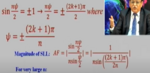
Hello,In a broad side array we have a radiation pattern which Array factor development shown bellow.
I can understand what is the problem that is called "grating lobe"
We bellow have th Array paatern expression howcan i see the grating lobe problem from it?
In the last photo we have an expression but i cant see the intuition of how to get it?
Thanks.

 

[Georgy.Moshkin]

Grating lobes have minimum when d=0.5*λ. From images below you can see that first grating lobe start to "grow" long before spacing reaches d=λ (in array factor). It is not the problem because antenna element factor will be low at that direction. If we continue to increase d, first grating lobe will move toward main lobe. At some point first grating lobe in array factor multiplied by element factor will result in significant peak in radiation pattern.

It's all about length of this portion in certain direction. Each antenna element will receive signal with
relative phase shift of 360*spacing*Cos(ang) (or length λ*spacing*Cos(ang)). When phase shift is 360° or λ then signals from two antenna elements will add in-phase in feeding network. When phase shift is 180° or 0.5*λ, then signals will add out of phase and become zero.

You can put these formulas in online calculator (configure plots as on my image below) https://mathnotepad.com/

phase(spacing,ang)=spacing*cos(ang)
sig_i(sp,ang)=cos(phase(sp,ang)*2*pi)
sig_q(sp,ang)=sin(phase(sp,ang)*2*pi)
sig(sp,ang)=abs(sig_i(sp,ang)+i*sig_q(sp,ang)+cos(0)+i*sin(0))
plot(sig(0.5,x/180*pi),sig(0.75,x/180*pi),sig(1,x/180*pi),sig(1.5,x/180*pi))
plot(phase(0.5,x/180*pi)*360,phase(0.75,x/180*pi)*360,phase(1,x/180*pi)*360)

Notice how grating lobe grows when spacing goes from d=0.5*λ to d=λ, and moved toward main lobe when spacing is d=1.5*λ

Grating lobes sometimes may be useful. For dual beam antennas you can optimize array factor to have grating lobes in desired directions and eliminate main lobe by designing radiation element with near zero element factor in broadside direction. AF with 3 lobes * element factor with 2 lobes = dual beam optimized gain antenna

 

[yefj]

Hello,assuming i dont want grating lobes.
I know that every element has a phase addition of distance*cos_theta
when each two elements has 0,360,720 phase between that meen that their radiation will be added.
So why each element has have a phase addition less then 2*pi to avoid some element to have constructive addition with some other element?
In radiation our beam pattern is formes by constructive addition of different radiation.
Or the meaning is that in broadside antenna the constructive addithin happens only at theta=90?
Thanks.

 

[Georgy.Moshkin]

d<λ - avoiding phase wrap around
d>n*λ - new grating lobe emerges for each n*λ (phase wrap around)
After d>λ relative element phases start to wrap around through 180° and 360°, giving zeroes and peaks.
It all comes from summation, try to consider trigonometry regardless antenna design.
You have N inputs of same frequency tone with certain phase offset.
If you want to understand how radiation is added intuitively, I think it is better to use more "low level" approach without using all "simplifications" from antenna theory books.
Assume we have patch at position (x1,y1,z1) and some point in space where we measure field (x2,y2,z2). All coordinates are normalized to wavelength λ. Distance between these points is d1(x1,y1,z1,x2,y2,z2)=Sqrt( (x2-x1)^2+(y2-y1)^2+(z2-z1)^2)
Then signal from each antenna signal with phase shift in exponential form for all those distances may be written as sig[N]=Exp(i*d1(x1[N],y1[N],z1[N],x2,y2,z2)*2*Pi)
And after summation of all sig[N] for N patches you can calculate 20*Log10(Abs(...)) of this sum to get radiation pattern value for point x2,y2,z2.

Here is another example (with less math). Let's call it "two points example":

Imagine first point in front of antenna at distance of 100 meters. For all patches distances to this point is almost the same, so phase shift will be almost the same (360*distance/λ=360*100/λ), which provides almost 0° relative phase shift (constructive addition)

Imagine second point, and put it on the left relative to antenna, at a distance of 100 meters.
If elements spacing is 0.5*λ then relative phase between adjacent patches will be 100+0.5*λ, 100+0.5*λ+0.5*λ, 100+0.5*λ+0.5*λ+0.5*λ and so on. 100 meters distance is the same for all patches, we only need relative offsets, which are 0.5*λ, 0.5*λ+0.5*λ, 0.5*λ+0.5*λ+0.5*λ.

If you imagine point smoothly moving from first position to second position (through a quarter-circle trajectory), then you will see how relative phase shift increases over angle.
point1: 0, 0, 0 (in front of antenna)
point2: 0.5*λ, 0.5*λ+0.5*λ, 0.5*λ+0.5*λ+0.5*λ (on the left side, rotated 90deg relative to broadside)

If d=1*λ point2 will have grating lobe, but element factor of radiator improves situation, because radiation is very weak at this direction:
point2: 1*λ, 1*λ+1*λ, 1*λ+1*λ+1*λ (constructive addition for the point on the left, the same as at broadside)

if d>λ, then point2: 1*λ, 1*λ+1*λ, 1*λ+1*λ+1*λ situation will emerge earlier, at some smaller angle, and start to be a problem.
Depending on element spacing d constructive addition may occur at several angles, not only at 90°.

If somebody read this later, please note that some sources use 90° (angle changes from 0° to 180°) for broadside and other use 0° for broadside (angle changes from -90° to 90°). And formula for spacing*cos(ang) will use sin(ang) if angle is measured relative to broadside axis.

 

[yefj]

Hello Georgy,I have tried to implement your words into full mathematical example as shown bellow.

i understand that grating lobe happen when two elements get the same phase for example 10 and 10+360=370
could you please guide me ragarding how to update my example so i will see grating lobe with the main lobe?
Thanks.

 

[Georgy.Moshkin]

I think that the first grating lobe appears at angles 90°±2*ASin(1/(2*d))*180°/Pi
where d is distance between elements (normalized) and main beam is at 90°
This formula gives right side lobe angles for graphs in post N2 (side lobes around 51° and 128° for 1.5*λ )
But needs to be rechecked.
p.s. d=distance in [mm] / λ [mm]

 

[yefj]

Hello Gorgy,i this i succseeded i just played with the formula in matlab and saw lobes in different angles.
The cosinus wave gets tighter but it represents the lobes.

x=-180:0.01:180;
x_rad=(pi/180).*x;
y=cos(2*pi*x_rad);
plot(x,y)