[SOLVED] MATLAB Waveguide Coupler Chebyshev Directivity Plot

[eefundi]

Hello again,

I have been stuck designing Chebyshev couplers and decided to go back to David Pozar's Microwave Engineering to reproduce his plots.

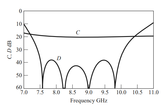
I am currently attempting to reproduce the below plot from example 7.4 on four-hole Chebyshev couplers (page 341, fourth edition).

Four-hole Chebyshev coupler plot from Pozar's book.

​

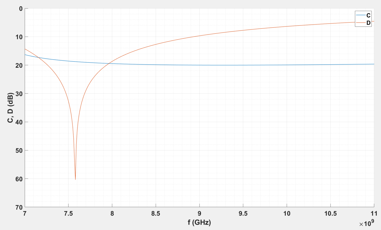
Of course, I tried to simulate this coupler in HFSS, but the results were very different. I figured I should first reproduce this theoretical pattern. I wrote the MATLAB code at the bottom of this post from which I obtained the plot below:

Plot obtained from MATLAB using same equations and values as the example.

​

This plot is very different from Pozar's. I have been stuck on this for so long, rechecking my code and so on. Even if there's an issue in the code, I probably can't find it because of how long I've spent on this.
I am starting to think that the issue may be in Pozar's book, as I noticed some other mistakes. For instance in example 7.3, the following calculations are written:

\[ 0.1 = 1.44 \times 10^{6} \cdot r_0^3 \quad \rightarrow \quad r_0 = 4.15 \ mm \]​

Although calculating for the radius with the same values gives \( r_0 = 4.11 \ mm \).

Either way, below is the MATLAB code for example 7.4. I would appreciate any comments.

clear; clc;
format long g

C = 20; D_m = 40; N = 3;
a=22.86.*10.^(-3); b=10.16.*10.^(-3);


%%%% Calculations at Operating Frequency %%%%

f_op = (9).*10.^9;
k_0 = 2.*pi.*f_op./(3.*10.^8); lambda_0 = (3.*10.^8)./f_op;

beta = sqrt(k_0.^2 - (pi./a).^2);
d = a/4;
lambda_g = 2.*pi./beta;
spacing = lambda_g./4;

T_f = -1j.*((2.*(k_0).^2)./(3.*beta.*a.*b)).*((sin((pi.*d)./(a))).^2) + 1j.*((4./(3.*a.*b))).*((beta.*(sin((pi.*d)./(a))).^2) + ((((pi).^2)./(beta.*a.^2))).*(cos((pi.*d)./(a))).^2);
T_b = -1j.*((2.*(k_0).^2)./(3.*beta.*a.*b)).*((sin((pi.*d)./(a))).^2) - 1j.*((4./(3.*a.*b))).*((beta.*(sin((pi.*d)./(a))).^2) - ((((pi).^2)./(beta.*a.^2))).*(cos((pi.*d)./(a))).^2);
T_b_abs = abs(T_b); T_f_abs = abs(T_f);

% the two equations above for the forward and backward wave coefficients
% are slightly different from those in Pozar's book. I used the equations
% from Collin's book, but they are essentially the same.

phi = (1./N).*acosh(10.^(D_m./20));
theta_m = acos(1./(cosh(phi)));

T_N = chebyshevT(N, sec(theta_m));
K = (10.^(-(C)./(20)))./(T_f_abs .* T_N);

r_0 = 3.26*10^(-3);
r_1 = 4.51*10^(-3);
r_2 = r_1; r_3 = r_0;

theta_upper = pi - theta_m;

f_lower = ((3.*10.^8)./(2.*pi)).*(sqrt(((((2.*beta)./(pi).*theta_m).^2)+((pi./a).^2))));
f_upper = ((3.*10.^8)./(2.*pi)).*(sqrt(((((2.*beta)./(pi).*theta_upper).^2)+((pi./a).^2))));


%%%% Sweep Calculations %%%%

f_sweep = 7*10^9:0.01*10^9:11*10^9;

k_s = 2.*pi.*f_sweep./(3.*10.^8); lambda_0_s = (3.*10.^8)./f_sweep;
beta_s = sqrt(k_s.^2 - (pi./a).^2);
lambda_gs = 2.*pi./beta_s;


T_f_s = -1j.*((2.*(k_s).^2)./(3.*beta_s.*a.*b)).*((sin((pi.*d)./(a))).^2) + 1j.*((4./(3.*a.*b))).*((beta_s.*(sin((pi.*d)./(a))).^2) + ((((pi).^2)./(beta_s.*a.^2))).*(cos((pi.*d)./(a))).^2);
T_f_abs_s = abs(T_f_s);

T_b_s = -1j.*((2.*(k_s).^2)./(3.*beta_s.*a.*b)).*((sin((pi.*d)./(a))).^2) - 1j.*((4./(3.*a.*b))).*((beta_s.*(sin((pi.*d)./(a))).^2) - ((((pi).^2)./(beta_s.*a.^2))).*(cos((pi.*d)./(a))).^2);
T_b_abs_s = abs(T_b_s);


C_sweep = -20.*log10(K.*T_f_abs_s.*abs(chebyshevT(N, sec(theta_m))));
% D_sweep = - C_sweep - 20.*log10(T_b_abs_s) - 20.*log10(K*abs(chebyshevT(N, sec(theta_m)*cos(beta_s*d))));
D_sweep = 20*log10(T_f_abs_s./T_b_abs_s) + 20*log10(chebyshevT(N, sec(theta_m))./( chebyshevT(N, sec(theta_m)*cos(beta*d)) ));

% D_sweep = 20*log10(T_f_abs./T_b_abs) + 20*log10(chebyshevT(N, sec(theta_m))./( chebyshevT(N, sec(theta_m)*cos(beta*d)) ));

sum_r = 0;
r_array = [r_0, r_1, r_2, r_3];
for i = 1:2
    sum_r = sum_r + ((r_array(i))^3)*(cos((N-2*i)*beta_s*d));
end



%%%% Plots %%%%

hold on;
plot(f_sweep, C_sweep, 'LineWidth', 1)
plot(f_sweep, D_sweep, 'LineWidth', 1)
set(gca, 'fontweight', 'bold','fontsize', 20, 'YDir','reverse')
xlabel('f (GHz)', 'fontsize',22)
ylabel('C, D (dB)', 'fontsize', 22)
legend('C', 'D')
hold off; grid on; grid minor;set(figure(1), 'Position', [100 100 800 500]);

Thanks,

Fundi

 

[eefundi]

Alright, code had an error where I used the wrong variable when calculating the coupling factor and directivity. I should have multiplied the swept beta by the spacing of the apertures, but I confused it with the aperture offset.

The corrected code and plot are below.

clear; clc;
format long g

%%%% Constants %%%%

C = 20; D_m = 40; N = 3;
a=22.86.*10.^(-3); b=10.16.*10.^(-3);
Z_10 = 550.9;
P_10 = (a.*b)./Z_10;
eta_0 =  120*pi;


%%%% Calculations at Operating Frequency %%%%

f_op = (9).*10.^9;
k_0 = 2.*pi.*f_op./(3.*10.^8); lambda_0 = (3.*10.^8)./f_op;
beta = sqrt(k_0.^2 - (pi./a).^2);
d = a./4;
lambda_g = 2.*pi./beta;
spacing = lambda_g./4;

T_f = -1j.*((2.*(k_0).^2)./(3.*beta.*a.*b)).*((sin((pi.*d)./(a))).^2) + 1j.*((4./(3.*a.*b))).*((beta.*(sin((pi.*d)./(a))).^2) + ((((pi).^2)./(beta.*a.^2))).*(cos((pi.*d)./(a))).^2);
T_b = -1j.*((2.*(k_0).^2)./(3.*beta.*a.*b)).*((sin((pi.*d)./(a))).^2) - 1j.*((4./(3.*a.*b))).*((beta.*(sin((pi.*d)./(a))).^2) - ((((pi).^2)./(beta.*a.^2))).*(cos((pi.*d)./(a))).^2);

phi = (1./N).*acosh(10.^(D_m./20));
theta_m = acos(1./(cosh(phi)));

T_N = chebyshevT(N, sec(theta_m));
K = (10.^(-(C)./(20)))./(abs(T_f) .* T_N);

r_0 = 3.26.*10.^(-3);
r_1 = 4.51.*10.^(-3);
r_2 = r_1; r_3 = r_0;

theta_upper = pi - theta_m;

f_lower = ((3.*10.^8)./(2.*pi)).*(sqrt(((((2.*beta)./(pi).*theta_m).^2)+((pi./a).^2))));
f_upper = ((3.*10.^8)./(2.*pi)).*(sqrt(((((2.*beta)./(pi).*theta_upper).^2)+((pi./a).^2))));


%%%% Sweep Calculations %%%%

f_sweep = 7.*10.^9:0.01.*10.^9:11.*10.^9;

k_s = 2.*pi.*f_sweep./(3.*10.^8); lambda_0_s = (3.*10.^8)./f_sweep;
beta_s = sqrt(k_s.^2 - (pi./a).^2);

T_f_s = -1j.*((2.*(k_s).^2)./(3.*beta_s.*a.*b)).*((sin((pi.*d)./(a))).^2) + 1j.*((4./(3.*a.*b))).*((beta_s.*(sin((pi.*d)./(a))).^2) + ((((pi).^2)./(beta_s.*a.^2))).*(cos((pi.*d)./(a))).^2);
T_b_s = -1j.*((2.*(k_s).^2)./(3.*beta_s.*a.*b)).*((sin((pi.*d)./(a))).^2) - 1j.*((4./(3.*a.*b))).*((beta_s.*(sin((pi.*d)./(a))).^2) - ((((pi).^2)./(beta_s.*a.^2))).*(cos((pi.*d)./(a))).^2);

% alternate equations for forward and backward waves coefficients. Should theoretically give same result, but somehow differ. %
% k_f_s = ((2.*k_s)./(3.*(eta_0).*P_10)).*(((sin((pi.*d)./(a))).^2) - ((2.*(beta_s).^2)./((k_s).^2)).*(((sin((pi.*d)./(a))).^2) + ((pi.^2)./((beta_s.^2).*(a.^2))).*(cos((pi.*d)./(a))).^2));
% k_b_s = ((2.*k_s)./(3.*(eta_0).*P_10)).*(((sin((pi.*d)./(a))).^2) + ((2.*(beta_s).^2)./((k_s).^2)).*(((sin((pi.*d)./(a))).^2) - ((pi.^2)./((beta_s.^2).*(a.^2))).*(cos((pi.*d)./(a))).^2));

cheby_var = sec(theta_m).*cos(beta_s.*spacing);

C_sweep = -20.*log10(K.*abs(T_f_s).*abs(chebyshevT(N, sec(theta_m))));
D_sweep = 20.*log10(abs(T_f_s./T_b_s)) + 20.*log10(abs(chebyshevT(N, sec(theta_m))./(chebyshevT(N, cheby_var))));


%%%% Plots %%%%

hold on;
axis([7.*10.^9 11.*10.^9 0 60])
plot(f_sweep, C_sweep, 'LineWidth', 3)
plot(f_sweep, D_sweep, 'LineWidth', 3)
set(gca, 'fontweight', 'bold','fontsize', 20, 'YDir','reverse')
xlabel('f (GHz)', 'fontsize',22)
ylabel('C, D (dB)', 'fontsize', 22)
legend('C', 'D')
hold off; grid on; grid minor;set(figure(1), 'Position', [100 100 800 500]);

Thanks,

Fundi