Plotting characteristics curve of Phase-frequency detector (PFD)

pancho_hideboo · Oct 23, 2015

See #17.
Remove ARTIST and PSF.
Set POST.

rafgamo · Oct 23, 2015

Remove ARTIST and PSF.
Set POST

I did what you said, then the only difference with the previous simulation is there is a .sn0 now

rafgamo · Oct 23, 2015

Code:

.option POST
.temp 25
.GLOBAL gnd! vdd!

.param fund_period=2n
.param delta_phase_deg=0.0
.param tdelay='(delta_phase_deg/360)*fund_period'

xi12 vdd! down up out_clk ref_clk start pfdv2_sch
v17 start gnd! dc=0 pulse ( 0 1.8 500p 1p 0 0.5 1)

v16 out_clk gnd! dc=0 pulse(0 1.8 '1.1*fund_period+tdelay'
+ 5p 5p 'fund_period/2' fund_period)

v2  ref_clk gnd! dc=0 pulse(0 1.8 '1.1*fund_period'
+ 5p 5p 'fund_period/2' fund_period)

v5 vdd! gnd! dc=1.8
c18 vctrl- gnd! c=.8p
c7 vctrl+ gnd! c=.8p
xi17 down up vctrl+ vctrl- cpv2_sch

.tran .1n 75n start=0
.sn tres='fund_period/10' period=fund_period
+ trinit='5*fund_period' maxtrinitcycles=5
+ sweep delta_phase_deg lin 101 -360 360
.op All 0
.option opfile=1 split_dp=1

.probe i1(c7)
.probe i2(c18)
.end

pancho_hideboo · Oct 23, 2015

rafgamo said:
I did what you said, then the only difference with the previous simulation is there is a .sn0 now

Show me time domain waveform of ref_clk and out_clk of .sn0.
I don't mean .tr0.

rafgamo said:

Try
.probe snfd i(c7)[0]
.probe snfd ir(c7)[0]
.probe snfd i(c18)[0]
.probe snfd ir(c18)[0]

rafgamo · Oct 23, 2015

Show me time domain waveform of ref_clk and out_clk of .sn0

Try
.probe snfd i(c7)[0]
.probe snfd ir(c7)[0]
.probe snfd i(c18)[0]
.probe snfd ir(c18)[0]

I also tried putting this into the netlist and got a .snf0 file

pancho_hideboo · Oct 23, 2015

pancho_hideboo said:
Show me time domain waveform of ref_clk and out_clk of .sn0.
I don't mean .tr0.

I confirmed you come to be able to sweep phase difference between ref_clk and out_clk.

rafgamo said:
I also tried putting this into the netlist and got a .snf0 file

Show me results.

rafgamo · Oct 23, 2015

Here,

Maybe this screenshot could help.

pancho_hideboo · Oct 23, 2015

Try plot ir1(c18)

0) and ir1(c7)

0).
And show me plot results.

rafgamo · Oct 23, 2015

Here

pancho_hideboo · Oct 23, 2015

Show me time domain waveform of i(c18) and i(c7) of .sn0.
Here you have to insert followings.
.probe i(c18) i(c7)

rafgamo · Oct 23, 2015

Show me time domain waveform of i(c18) and i(c7) of .sn0

But can't see any i(c18) and i(c7).

I already inserted the .probe i(c18) i(c7) as what you advised.

Code:

.option PARHIER = LOCAL

.option POST
.temp 25

.GLOBAL gnd! vdd!

.param fund_period=2n
.param delta_phase_deg=0.0
.param tdelay='(delta_phase_deg/360)*fund_period'


xi12 vdd! down up out_clk ref_clk start pfdv2_sch
v17 start gnd! dc=0 pulse ( 0 1.8 500p 1p 0 0.5 1)

v16 out_clk gnd! dc=0 pulse(0 1.8 '1.1*fund_period+tdelay'
+ 5p 5p 'fund_period/2' fund_period)

v2  ref_clk gnd! dc=0 pulse(0 1.8 '1.1*fund_period'
+ 5p 5p 'fund_period/2' fund_period)

v5 vdd! gnd! dc=1.8
c18 vctrl- gnd! c=.8p
c7 vctrl+ gnd! c=.8p
xi17 down up vctrl+ vctrl- cpv2_sch

.tran .1n 75n start=0
.sn tres='fund_period/10' period=fund_period
+ trinit='5*fund_period' maxtrinitcycles=5
+ sweep delta_phase_deg lin 101 -360 360
.op All 0
.option opfile=1 split_dp=1

.probe i1(c7)
.probe i1(c18)
.probe snfd i(c7)[0]
.probe snfd ir(c7)[0]
.probe snfd i(c18)[0]
.probe snfd ir(c18)[0]
.probe i(c18) i(c7)
.end

pancho_hideboo · Oct 23, 2015

Sorry try
.probe sn i(c18) i(c7)

.probe snfd i(18) i(c7)
.probe snfd i(18)[0] i(c7)[0]

.probe snfd ir(c18) ir(c7)
.probe snfd ir(c18)[0] ir(c7)[0]

Plot i(c18) and i(c7) of "input.sn0".

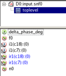
Your results of ir1(c18)

0) and ir1(c7)

0) are both extraordinary.

Plot i(c18) and i(c7) of "input.snf0", here you have to select real() and index=0 from Custom waveView.

Try inseart follwing into netlist.
.measure sn In AVG i(c18)
.measure sn Ip AVG i(c7)
.measure sn Ipump param='In+Ip'
And plot them. Show me results.

rafgamo · Oct 23, 2015

Plot i(c18) and i(c7) of "input.sn0"

Plot i(c18) and i(c7) of "input.snf0"

here you have to select real() and index=0 from Custom waveView

I'm not sure if I did it right.

- - - Updated - - -

Plots for In, Ip and Ipump.

pancho_hideboo · Oct 23, 2015

Plot i(c18) and i(c7) of "input.sn0" are reasonable.

Try following

Code:

.sn tone='1/fund_period' nharms=10
+ trinit='5*fund_period' maxtrinitcycles=5
+ sweep delta_phase_deg lin 101 -360 360

instead of

Code:

.sn tres='fund_period/10' period=fund_period
+ trinit='5*fund_period' maxtrinitcycles=5
+ sweep delta_phase_deg lin 101 -360 360

Then plot ir1(c18)

0) and ir1(c7)

0) of .snf0.

You use "HSPICE RF -- D-2010.03-SP2 (Aug 26 2010)".
It is relative old.
Do you have newer version ?

rafgamo · Oct 23, 2015

Then plot ir1(c18)0) and ir1(c7)0) of .snf0

You use "HSPICE RF -- D-2010.03-SP2 (Aug 26 2010)".
It is relative old.
Do you have newer version ?

Yeah its pretty old, and its the only version our school provides.

pancho_hideboo · Oct 23, 2015

In #29, x-axis is phase from -360 to 360.

Since you sweep "delta_phase_deg",
dependencies of data in "*.sn0" are [delta_phase_deg, time],
dependencies of data in "*.snf0" are [delta_phase_deg, harmonic_index].

For example, ir1(c1):0 in "*.snf0" mean real part of i1(c1) for harmonic_index=0,
so its dependecy, that is, x-axsis is "delta_phase_deg".
However it is not in #35.

Show me netlist again.

Example
For a demonstration of using Shooting Newton analysis you can run the pdfcpGain.sp file shipped with the HSPICE RF distribution, located in the directory $<installdir>/hspicerf/examples.
This example performs analysis on a D-flipflop phase frequency divider with charge pump, implemented in 50nm technology.
The example is configured to measure the gain (volts per degree) of the DFF PFD and tri-state output combination.

rafgamo · Oct 23, 2015

Code:

.option PARHIER = LOCAL

.option POST
.temp 25

.GLOBAL gnd! vdd!

.param fund_period=2n
.param delta_phase_deg=0.0
.param tdelay='(delta_phase_deg/360)*fund_period'

xi12 vdd! down up out_clk ref_clk start pfdv2_sch
v17 start gnd! dc=0 pulse ( 0 1.8 500p 1p 0 0.5 1)

v16 out_clk gnd! dc=0 pulse(0 1.8 '1.1*fund_period+tdelay'
+ 5p 5p 'fund_period/2' fund_period)

v2  ref_clk gnd! dc=0 pulse(0 1.8 '1.1*fund_period'
+ 5p 5p 'fund_period/2' fund_period)

v5 vdd! gnd! dc=1.8
c18 vctrl- gnd! c=.8p
c7 vctrl+ gnd! c=.8p
xi17 down up vctrl+ vctrl- cpv2_sch

.tran .1n 75n start=0
.sn tone='1/fund_period' nharms=10
+ trinit='5*fund_period' maxtrinitcycles=5
+ sweep delta_phase_deg lin 101 -360 360

.op All 0
.option opfile=1 split_dp=1

.probe i1(c7)
.probe i1(c18)
.probe snfd i(c7)[0]
.probe snfd i(c18)[0]
.probe snfd i(c18) i(c7)
.probe snfd i(c18)[0] i(c7)[0]

.probe snfd ir(c18)[0]
.probe snfd ir(c7)[0]
.probe snfd ir(c18) ir(c7)
.probe snfd ir(c18)[0] ir(c7)[0]

.probe sn i(c18) i(c7)

.measure sn Ip AVG i(c18)
.measure sn In AVG i(c7)
.measure sn Ipump param='In+Ip'

.end

pancho_hideboo · Oct 23, 2015

.probe i1(c7)
.probe i1(c18)
.probe snfd i(c7)[0]
.probe snfd i(c18)[0]
*.probe snfd i(c18) i(c7)
*.probe snfd i(c18)[0] i(c7)[0]

.probe snfd ir(c18)[0]
.probe snfd ir(c7)[0]
*.probe snfd ir(c18) ir(c7)
*.probe snfd ir(c18)[0] ir(c7)[0]

.probe sn i(c18) i(c7)

rafgamo · Oct 24, 2015

I inserted the lines in #38... Here is the plot for ir1(c18)

0) and ir1(c7)

0) of .snf0

pancho_hideboo · Oct 24, 2015

Plot i1(c7):0 and i1(c18):0.

Welcome to EDAboard.com

Plotting characteristics curve of Phase-frequency detector (PFD)

Advanced Member level 5

Member level 1

Member level 1

Advanced Member level 5

Member level 1

Advanced Member level 5

Member level 1

Advanced Member level 5

Member level 1

Advanced Member level 5

Member level 1

Attachments

Advanced Member level 5

Member level 1

Advanced Member level 5

Member level 1

Advanced Member level 5

Member level 1

Advanced Member level 5

Member level 1

Advanced Member level 5

Similar threads

Part and Inventory Search

Welcome to EDABoard.com

Sponsor