Circuit Performance Exploration

[melkord]

My supervisor suggested me to do some performance exploration of a circuit (using optimization feature in Cadence).
So the starting point I have is only the topology without any specific target specification.
The main goal is to find the "border" or limit of performance of this specific circuit.

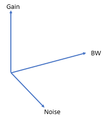
In my mind, I would get something like the picture below.
Gain, BW, and Noise are just an example.
They could be other circuit performance.

Could someone briefly inform me how it is usually done?
I would also really appreciate it if someone can point me to any reference about this.

 

[jjx]

Usually is perhaps a strong word, but it spans from/over using the expertise of the designer, time-to-market, brute-force monte-carlo, genetic algorithms, optimization tools, etc.

With that said, there are also plenty of papers out there of various detail. But use search words as operational amplifier genetic and neural networks and cadence own optimizer descriptions.

So, there have been many trials throughout the years and success rate has been somewhat limited as the holy graal more often is some other vague cost measure, like for example design time, deadline, "good-enough" mentality, etc.

To be honest, I tend to prefer brute force monte-carlo if I have the luxury of "free" licenses. Associate W, L, I with each transistor. Pick a random value from certain limits. Set up the simulation criteria (dc + tran + ac or so), evaluate and store the results. Then plot those meeting some kind of realistic specification in your x-dimensional graph. Not very academic nor very efficient, but satisfying and no extra brains required. An eight-transistor, two-stage operational amplifier with an RC miller compensation does not give you too many variables to juggle with, in the end.

 

[24BSNR]

Agree with jjx on the optimizers. They show a lot of promise, but there are a tremendous number of free design variables and hence permutations to have to sift through. On top of that setting up the optimization targets is not simple. This costs a lot of time to simulate which may or may not give one what you want.

Something that shows more promise IMO, is using Gm/Id approach, where you create large operating point tables of behavior around one device (nmos,pmos each) and can quickly grab results for optimization around predefined curves (see Jesper et. al).

There's also a text related to both, by David Binkley, "Tradoffs and optimization in Analog Design." He uses excel tables to design, with moderate inversion region as a design target (similar to gm/Id). Choosing a gm/Id target, quickly minimizes free design variables and speeds up the optimization.

 

[melkord]

Usually is perhaps a strong word, but it spans from/over using the expertise of the designer, time-to-market, brute-force monte-carlo, genetic algorithms, optimization tools, etc.

With that said, there are also plenty of papers out there of various detail. But use search words as operational amplifier genetic and neural networks and cadence own optimizer descriptions.

So, there have been many trials throughout the years and success rate has been somewhat limited as the holy graal more often is some other vague cost measure, like for example design time, deadline, "good-enough" mentality, etc.

To be honest, I tend to prefer brute force monte-carlo if I have the luxury of "free" licenses. Associate W, L, I with each transistor. Pick a random value from certain limits. Set up the simulation criteria (dc + tran + ac or so), evaluate and store the results. Then plot those meeting some kind of realistic specification in your x-dimensional graph. Not very academic nor very efficient, but satisfying and no extra brains required. An eight-transistor, two-stage operational amplifier with an RC miller compensation does not give you too many variables to juggle with, in the end.

Hello, could you explain more because I do not understand why I should use Monte Carlo simulation?
What I would like to know is the nominal limit of the circuit performance not the best/worst due to process variation.
As I understand it, Monte Carlo simulation works on one design, i.e., perturbs one design. Monte Carlo cannot show the nominal "border" or limit of performance of the circuit.
Monte Carlo simulation will show something like BW: 2MHz +/- 2kHz. However, it does not mean that the nominal border of the circuit are 1.998 MHz and 2.002 Mhz. Other example of nominal limit would be GBW is max in moderate inversion for a given power.

Agree with jjx on the optimizers. They show a lot of promise, but there are a tremendous number of free design variables and hence permutations to have to sift through. On top of that setting up the optimization targets is not simple. This costs a lot of time to simulate which may or may not give one what you want.

Something that shows more promise IMO, is using Gm/Id approach, where you create large operating point tables of behavior around one device (nmos,pmos each) and can quickly grab results for optimization around predefined curves (see Jesper et. al).

There's also a text related to both, by David Binkley, "Tradoffs and optimization in Analog Design." He uses excel tables to design, with moderate inversion region as a design target (similar to gm/Id). Choosing a gm/Id target, quickly minimizes free design variables and speeds up the optimization.

Hello, I am familiar with both books and still have difficulties to apply the method when what I need to find is the limit or border of the circuit performance instead of meeting a defined specification.
The picture below is an example what I have done before for a smaller circuit using the knowledge from those books.
The difficulties rise when there are many free variables, for example, in input-reffered offset voltage or in large circuits.
In input-reffered offset voltage, we have W and L in the formula, in addition of gm or gm/id.

 

[jjx]

Hello, could you explain more because I do not understand why I should use Monte Carlo simulation?
What I would like to know is the nominal limit of the circuit performance not the best/worst due to process variation.
As I understand it, Monte Carlo simulation works on one design, i.e., perturbs one design. Monte Carlo cannot show the nominal "border" or limit of performance of the circuit

Hi,

when I said Monte Carlo I was thinking of the method in it's original sense.

Monte Carlo method - Wikipedia

en.wikipedia.org

not the circuit-level monte-carlo (which essentially is the same, but yet).

Rather than optimizing or forlooping over parameters or whatever, you while-loop-forever a random process picking new W and L and I and V and what-have you within reasonable limits. Apply the simulation and get the results. You will eventually get a huge table with all random parameters and simulated results:

| W1 | W2 | L1 | L2 | CL | Itail | Iout | Vsup || A0 | w3db | wug | phim |  SR  |
+----+----+----+----+----+-------+------+------++----+------+-----+------+------+
|1.21|2.31|0.34|0.15|1.1p| 131.4u|432.1u| 2.49 || 13 | 10e6 |130e6| 43.2 | 10e6 |
+----+----+----+----+----+-------+------+------++----+------+-----+------+------+
...
+----+----+----+----+----+-------+------+------++----+------+-----+------+------+

Now you can find all extremes in the table, with simple queries

find(params, where SR > 8e6) & find(params, where A0 > 30) & ...

or scatterplot gain vs slew rate

plot(A0, SR)

or 3d-plot your original Gain vs Noise vs Bw.

plot(A0,Pn,Bw)

If you let the loop run forever, you will eventually get all the boundaries quite visible in your graph.

 

[melkord]

Rather than optimizing or forlooping over parameters or whatever, you while-loop-forever a random process picking new W and L and I and V and what-have you within reasonable limits. Apply the simulation and get the results. You will eventually get a huge table with all random parameters and simulated results:

| W1 | W2 | L1 | L2 | CL | Itail | Iout | Vsup || A0 | w3db | wug | phim |  SR  |
+----+----+----+----+----+-------+------+------++----+------+-----+------+------+
|1.21|2.31|0.34|0.15|1.1p| 131.4u|432.1u| 2.49 || 13 | 10e6 |130e6| 43.2 | 10e6 |
+----+----+----+----+----+-------+------+------++----+------+-----+------+------+
...
+----+----+----+----+----+-------+------+------++----+------+-----+------+------+

Now you can find all extremes in the table, with simple queries

find(params, where SR > 8e6) & find(params, where A0 > 30) & ...

or scatterplot gain vs slew rate

plot(A0, SR)

or 3d-plot your original Gain vs Noise vs Bw.

plot(A0,Pn,Bw)

If you let the loop run forever, you will eventually get all the boundaries quite visible in your graph.

Thank you for the explanation! I got the idea.
Do you think this can be done with Cadence?

 

[jjx]

Thank you for the explanation! I got the idea.
Do you think this can be done with Cadence?

If you have access to ADEXL you can. Not too complicated.

Define your variables (as globals). W1,W2, whatever.

Then create a model file with something like:

statistics {
process{
vary w1 dist=unif N=100 percent=yes
vary w2 dist=unif N=100 percent=yes
vary l1 dist=unif N=100 percent=yes
// ...
}
}

etc. Make sure to include that model file in the Setup > Models. Then launch a Montecarlo in Cadence.

Then you, however, have to find a clever way of plotting/filtering your results in cadence, but perhaps you can do an export to matlab/python or similar from the results / detail menu and utilize some more efficient plotting.

--- Updated May 31, 2022 ---

If you have access to ADEXL you can. Not too complicated.

Define your variables (as globals). W1,W2, whatever.

Then create a model file with something like:

statistics {
process{
vary w1 dist=unif N=100 percent=yes
vary w2 dist=unif N=100 percent=yes
vary l1 dist=unif N=100 percent=yes
// ...
}
}

etc. Make sure to include that model file in the Setup > Models. Then launch a Montecarlo in Cadence.

Then you, however, have to find a clever way of plotting/filtering your results in cadence, but perhaps you can do an export to matlab/python or similar from the results / detail menu and utilize some more efficient plotting.

And the above implies that w1 will be randomly selected between 0 and 2*(nominal global value) with a uniform distribution.

 

[dick_freebird]

Monte Carlo is for when you've got a surplus of time and
a defecit of clues, about what goes on. Figure that 90+%
of MC iterations tell you nothing useful other than "me too!".
And, to be useful, your MC infrastructure of individual param
statistics, param-param correlation and intra-param mismatch
all needs to be realistic.

Back in the good old days before CAD management weasels
told design management weasels that N=100 MC iterations
were a magic bean to get 100% line yield, I'd just put "k"
factors on critical params and nested-loop them. Doesn't
take a lot of points to deduce a trend. Step across the range
each, like *0.8, *0.9, *1.0, *1.1, *1.2 and you will get a close-in
"response surface" across the dimensions you exercised.
You can manipulate those in Parametric Analysis (Cadence)
or by looping in any SPICE control block.

You'll be ahead on effort, if you determine beforehand for
key transistors, what about them matters and how much
you can vary device geometry, sanely. Then I'd start from
the pins, back to front, as output attributes will set device
sizes and topology pretty authoritatively; then work back
along the signal chain to roughly-right-size each; then
start with the stimulus/response/conclusion loops.

 

[24BSNR]

Hello, I am familiar with both books and still have difficulties to apply the method when what I need to find is the limit or border of the circuit performance instead of meeting a defined specification.
The picture below is an example what I have done before for a smaller circuit using the knowledge from those books.
The difficulties rise when there are many free variables, for example, in input-reffered offset voltage or in large circuits.
In input-reffered offset voltage, we have W and L in the formula, in addition of gm or gm/id.

View attachment 176487

This is why I said you might have a huge number of parameters to sift through. Imagine you have a voffset with a granularity of 1uv and range of 50mv. That's 50,000 parameter points alone! Then you add in W,L etc... the search space grows large quickly. Like someone else pointed out, if computation and time was no problem you could easily try every permutation of the search space and get all the boundaries (called brute force, this also assumes each permutation has a functional simulation that works, they may not... eg.. bias could be improper). You could start with larger resolution like vos in range 1m to 50m in 1mv steps and look for a reasonable performance curve where you could interpolate over smaller regions. Or often, in machine learning and AI, they use heuristics to minimize the search space (maybe you know voffset will be very close to 10mv or less than 5mv, which drastically reduces the search space).

The beauty of the gm/id approach is you already have most of the numbers crunched in tables. You only need to set up your optimization properly to get a fast visual of the search space vs. parameters.

It might be easier to show exactly what you are trying to optimize to get a better idea of what you are trying to do.