DeboraHarry
Full Member level 5
I've tried to simulate a half-wave dipole in HFSS, using a perfect electrical conductor (pec). The dipole is 500 mm long in total, with a small gap between the two arms to allow a lumped port to be put there. So this should be a half-wave at 300 MHz.
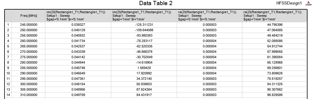
Using a wire radius of 1 mm, with a 1 mm gap between the terminals, the input impedance is 84 + j 51 Ohms. See 3rd and 5th colums below.

The impedance of an infinitely thin half-wave dipole is known to be 73 + j 42 Ohms, but since this is a finite thicknesss, I would expect the thickness to decrease the impedance somewhat, so 84 + j 51 Ohms makes no sence whatever to me.
If I change the wire radius to 0.1 mm, which should more closely approximate the theory for an infinitely thin dipole, and narrow the feed gap to 0.1 mm too, so the results go totally bizare - an input impedance of 0.000003 + j 0.05 Ohms. (See 2nd and 4th columns)
Can anyone see what's wrong with the model attached? The AirBox is sufficiently large to allow analysis down to 100 MHz, so I'm a bit puzzled why the results are so bizzare.
I find it quite worrying using HFSS. I often get results, and really have no idea if they are sensible or not. It is very easy to get incorrect results, and I personally find it hard to know when my model will introduce problems.
I used the Antenna Design kit (free download for HFSS uses) and synthesised a dipole with that. It chose a radius of 7.5 mm for a 300 MHz dipole, but in practice people will make them much thiner than that. But with my model, that gives an impedance of 106 + j 43. So whilst the imaginary part is about right, the real part is way off.
Of course, I could look at the design produced by the antenna design kit, and no doubt use that to get a better result for a half-wave dipole. But that just proves I can't get decent results myself, which is worrying.
Deborah
Using a wire radius of 1 mm, with a 1 mm gap between the terminals, the input impedance is 84 + j 51 Ohms. See 3rd and 5th colums below.
The impedance of an infinitely thin half-wave dipole is known to be 73 + j 42 Ohms, but since this is a finite thicknesss, I would expect the thickness to decrease the impedance somewhat, so 84 + j 51 Ohms makes no sence whatever to me.
If I change the wire radius to 0.1 mm, which should more closely approximate the theory for an infinitely thin dipole, and narrow the feed gap to 0.1 mm too, so the results go totally bizare - an input impedance of 0.000003 + j 0.05 Ohms. (See 2nd and 4th columns)
Can anyone see what's wrong with the model attached? The AirBox is sufficiently large to allow analysis down to 100 MHz, so I'm a bit puzzled why the results are so bizzare.
I find it quite worrying using HFSS. I often get results, and really have no idea if they are sensible or not. It is very easy to get incorrect results, and I personally find it hard to know when my model will introduce problems.
I used the Antenna Design kit (free download for HFSS uses) and synthesised a dipole with that. It chose a radius of 7.5 mm for a 300 MHz dipole, but in practice people will make them much thiner than that. But with my model, that gives an impedance of 106 + j 43. So whilst the imaginary part is about right, the real part is way off.
Of course, I could look at the design produced by the antenna design kit, and no doubt use that to get a better result for a half-wave dipole. But that just proves I can't get decent results myself, which is worrying.
Deborah
Attachments
Last edited:
") P).
P).