Continue to Site
Follow along with the video below to see how to install our site as a web app on your home screen.
Note: This feature may not be available in some browsers.
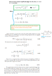
I just find an error in the expression after "rearranging".

As you can see in the attachment, the book is wrong, and the values are different depending on whether the two different Tau's are large or small in relation to each other. "k" is the ratio of one Tau to the other, and the final value of the term depends on whether k goes to infinity or zero.
is not right.the values are different depending on whether the two different Tau's are large or small in relation to each other.
If tau1, tau2 are positive and tau1 != tau2, the limits of the function are
lim f(t)=1
t->0
lim f(t)=0
t->inf
regardless wich one of tau1 or tau2 is greater
Furthermore if I swap tau1 and tau2 the shape of the function is still the same
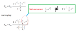
I mean that
is not right.
The final value (i.e. for t->Inf) of the expression is 0 for tau1<tau2 as well as for tau1>tau2, both >0 and finite.
Regards
Z
- - - Updated - - -
Oh, I had cross-posting with albbg!
The two tau's don't need to be very different. The limits given by albbg are valid anyway (with the only restrictions said in the previous posts).
Ratch,
Then, now I see that when you say "final value" you don't mean the value for t->inf, like many of us are used (see for example https://en.wikipedia.org/wiki/Final_value_theorem). You mean another thing, right? No problem.
It's clear that when tau1>>tau2 the expression approaches exp(-t/tau1) .
You get that result considering tau2=k*tau1 and looking the limit for k->0+ .
Now, let's see what happens when tau1<<tau2 .
To that end, please consider tau1=k*tau2 and consider the limit for k->0+ .
Obviously, the result is exp(-t/tau2) .
As pointed out by albbg in post #14, "if I swap tau1 and tau2 the shape of the function is still the same".
Regards
Z