bi2de matlab

Sampling
---------------------------
Converting an analog signal to a digital one is a necessary step for a computer to
analyze a signal: modern computers are digital machines, and can store only digital values.

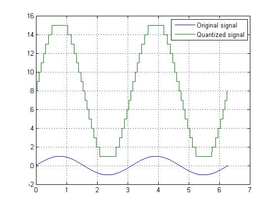
In the continuous function x(t), we replace t, the continuous variable, with nTs, a discrete value. We use n to index the discrete array, and Ts is the sampling period, the amount of time between two samples. The sampling time is the inverse of the sampling frequency fs, that is, Ts = 1/fs.

Before we can talk about sampling, let us call the frequency range of the signal
that we are interested in the bandwidth. Sometimes, we simply use the highest
frequency as the bandwidth, implying that we are interested in all frequencies between 0 Hz and the maximum. Other times, it may be limited, e.g., the visible light spectrum.

The term critical sampling applies to the case when the sampling rate is exactly twice the bandwidth, B. This means that we will record the signal just fast enough to properly reconstruct it later, i.e., fs = 2B. We get this value based on Nyquist's criterion, fs ≥2B, and choosing the lowest possible sampling frequency.

Oversampling is taking samples more frequently than needed (or more than 2 times the bandwidth). This results in more samples than are needed. You can use oversampling, but you may not want to due to hardware limitations, like not being able to process it fast enough, or not being able to store it in memory. Oversampling may be something you would want to do if you are working with cheap hardware, such as an inexpensive digital-to-analog converter, which appears to be the case with CD players. An inexpensive digital-to-analog converter may use a simple step function to recreate the signal. Therefore, the more samples it has to work with, the smaller the time between the samples, and the better it approximates the original. As a counter example, reading (and storing) the temperature every microsecond would produce a massive volume of data with no gain for predicting tomorrow's weather.

Undersampling occurs when we do not take samples often enough, less than twice the bandwidth. You would not want to use this, since you cannot reconstruct the signal. Also, any analysis done on an undersampled signal will likely be erroneous (as we say in computer programming, \garbage in, garbage out").

x[n] = x(nTs) describes the sampling process. Ts is the sampling time, while
n is an index. This means that the continuous signal x is converted into a digital
representation. x[n] is not exactly the same as x(t). It cannot be, since x(t) is
continuous. At best, x[n] is a good approximation of x(t).

The period of a signal is the length of time before it repeats itself. For a sinusoid,
we only need to know the frequency f, since we define the period as T = 1/f .

Example:
If we used x(t) below and sampled it at 20 kHz, how many samples would we have
after 60 ms?

x(t) = 3 cos(2Π404t +Π/4) + 2 cos(2Π6510) + cos(2Π660t -Π/5)

Answer:
The first thing to notice is that the number of samples really does not depend on
the signal itself. That is, all we need to answer this question is the 20 kHz sampling
rate (fs) and the total time 60 ms.

The sampling period is 1/(20 kHz) or 1/(20,000 Hz). Since Hz is in cycles/sec,
1/Hz would be sec/cycles, or just seconds. We take the first sample at time = 0,
then wait 1/(20,000) sec, and take another, and continue until 60 ms = 0.060 seconds is up.

To find the numerical answer, multiply 0.060 by 20,000, then add 1 (since the
first sample was taken at time 0). For answering this (or any) question on a test,
it is important to show your thought process. A good answer would include the
analysis (and wording) as above.

Thanks

Hi everybody,

Theory (DSProakis)
x[n]=x(nT) here, in CT (continous time)signal t = nT, to get DT (Discrete time)sequence
if x(t)=cos(2*pi*F*t) where F is the analog freq.
discrete seq x[n]=x(nT)=cos(2*pi*F*n*T)
T=sampling interval=1/Fs , Fs=sampling rate (samples/sec) n=No.of samplesof x[n]=N
x[n]=x(nT)=cos(2*pi*F*n*T)=cos(2*pi*n*F/Fs)
where, discrete freq f = F/Fs ;

Programming tips:

Note:1
No. of cycles in x[n] = ( n*F)/Fs = total no. of periods in x[n]

Note:2
no. of samples/period = n / ( n*F/Fs ) = Fs / F = No. of samples in 1 period.

Note:3
t = 0 : sampleInterval : seconds;
where seconds / sampleInterval = the number of samples per second
t = 0 : (1/Fs) : (0:N-1)/Fs ; where N = n = no.of samples in x[n]
therefore, length(x)=length(t)

Note:4
The signal x[n] will have a length, in time of (n/Fs) seconds.
i.e, the time variable "t" varies between 0 to n/Fs.= total time of the signal x[n].


happy learning

x[n] = x(nts) matlab

Bit to Symbol Mapping:

in matlab we can convert binary vectors to decimal numbers by using the command bi2de as follows;

d = bi2de(b)
d = bi2de(b,flg)
d = bi2de(b,p)
d = bi2de(b,p,flg)

Description

d = bi2de(b) converts a binary row vector b to a nonnegative decimal integer. If b is a matrix, each row is interpreted separately as a binary number. In this case, the output d is a column vector, each element of which is the decimal representation of the corresponding row of b.

d = bi2de(b,flg) is the same as the syntax above, except that flg is a string that determines whether the first column of b contains the lowest-order or highest-order digits. Possible values for flg are 'right-msb' and 'left-msb'. The value 'right-msb' produces the default behavior.

d = bi2de(b,p) converts a base-p row vector b to a nonnegative decimal integer , where p is an integer greater than or equal to 2. The first column of b is the lowest base-p digit. If b is a matrix, the output d is a nonnegative decimal vector, each row of which is the decimal form of the corresponding row of b.

d = bi2de(b,p,flg) is the same as the syntax above, except that flg is a string that determines whether the first column of b contains the lowest-order or highest-order digits. Possible values for flg are 'right-msb' and 'left-msb'. The value 'right-msb' produces the default behavior.

Examples

The code below generates a matrix that contains binary representations of five random numbers between 0 and 15. It then converts all five numbers to decimal integers.

b = randint(5,4); % Generate a 5-by-4 random binary matrix.
de = bi2de(b);
disp(' Dec Binary')
disp(' ----- -------------------')
disp([de, b])

Sample output is below. Your results might vary because the numbers are random.

Dec Binary
----- -------------------
13 1 0 1 1
7 1 1 1 0
15 1 1 1 1
4 0 0 1 0
9 1 0 0 1

The command below converts a base-five number into its decimal counterpart, using the leftmost base-five digit (4 in this case) as the most significant digit. The example reflects the fact that 4(5^3) + 2(5^2) +5^0 = 551.

d = bi2de([4 2 0 1],5,'left-msb')

The output is

d =

551

here you are another examples:

%convert the bits in x into k-bit symbols
x=randint(20,1,2); %Generate 20 binary numbers.
x_reshaped=reshape(x,5,4); %reshape x to be 5-by-4 matrix, each 4-bits
%putted in one row to create 5 rows each of
%4-bits.
x_decimal=bi2de(x_reshaped,'left-msb');
x_decimal_as_row=x_decimal'
stem(x_decimal_as_row),grid; %plot the symbols;


Example:

x=randint(100,1,2);
x_shd=reshape(x,25,4);
x_dec=bi2de(x,'left-msb');
stem(x_dec),grid;


Example:

x=rand(100,1)>0.5; %generate 100 binary digits
x2=reshape(x,20,5);
decimal=bi2de(x2,'left-msb');
stem(decimal(1:10)); %stem plot for first 10 decimal numbers.

Enjoy

Now we can plot the Fourier series representation using MATLAB and see how
the series does at reproducing the original signal. If we plot the ¯rst 20 terms in the sum, we see the general shape of the original function but we see a lot of 'ringing'. As we plot more terms, we see the original function is represented quite accurately. In general Fourier series can reconstruct a signal with a small number of modes if the original signal is smooth. Discontinuities require many high frequency components to construct the signal accurately.

For reference, the MATLAB code that generated this figure is given below:

N = 20;
x = [0:100]/100;
f = ones(1,101)*1/2;
for i = 1:2:N
a = 2/pi/i;
f = f+ a*sin(2*pi*i*x);
end
plot(x,f,'r'),axis([-.5 1.5 0 1.5]);grid



Enjoy

This is a program in Matlab to do the DFT and the FFT (2-sided and 1-sided)

Good luck
%FFT lecture.
clc;close all; clear all;
%Generate the sine wave sequences
fs=8000; % sampling rate
N=1000; % Number of data points.
x=2*sin(2000*pi*[0:1:N-1]/fs) ;
figure(1) ;
stem( 1 : 1:N/10,x( 1 : 1 :N/10 ) ,'filled' ) ;%plot first 100 sample of x
%% Apply the DFT algorithm
figure(2) ;
xf=abs(fft(x) )/N;% compute the amplitude spectrum
P=xf.*xf;%compute the power spectrum
% Map the frequency bin to the frequency (hz)
f=[0:1:N-1]*fs/N;%fk=k fs/N where k=0,1,2,...N-1
% now we will plot the DFT spectrums
subplot(211);plot(f,xf);grid
xlabel('Frequency (Hz)');ylabel('Amplitude Spectrum (DFT) ' ) ;
subplot(212);plot(f,P);grid
xlabel('Frequency (Hz)');ylabel('Power Spectrum (DFT) ' ) ;
%% Convert it to one sided spectrum
figure(3);
xf(2:N)=2*xf(2:N);%Get the single side spectrum
P=xf.*xf;%compute the power spectrum
% Map the frequency bin to the frequency (hz)
f=[0:1:N/2]*fs/N;%frequency up to the folding frequency fs/2
% now we will plot the DFT spectrums
subplot(211);plot(f,xf(1:N/2+1));grid
xlabel('Frequency (Hz)');ylabel('Amplitude Spectrum (DFT)');
title('One Sided-Spectrum')
subplot(212);plot(f,P(1:N/2+1));grid
xlabel('Frequency (Hz)');ylabel('Power Spectrum (DFT)');
title('One Sided-Spectrum')
%% Zero Padding to the length of 1024
figure(4);
x=[x,zeros(1,24)];%24 zero to extend the sequence x from 1000 to 1024
N=length(x);
xf=abs(fft(x))/N; %compute the amplitude spectrum with zero padding
P=xf.*xf;%compute the power spectrum
% Map the frequency bin to the frequency (hz)
f=[0:1:N-1]*fs/N;%fk=k fs/N where k=0,1,2,...N-1
subplot(211);plot(f,xf);grid
xlabel('Frequency (Hz)');ylabel('Amplitude Spectrum (FFT)');
subplot(212);plot(f,P);grid
xlabel('Frequency (Hz)');ylabel('Power Spectrum (FFT)');
%% Convert it to one sided spectrum
figure(5);
xf(2:N)=2*xf(2:N);%Get the single side spectrum
P=xf.*xf;%compute the power spectrum
% Map the frequency bin to the frequency (hz)
f=[0:1:N/2]*fs/N;%frequency up to the folding frequency fs/2
% now we will plot the FFT spectrums
subplot(211);plot(f,xf(1:N/2+1));grid
xlabel('Frequency (Hz)');ylabel('Amplitude Spectrum (FFT)');
title('One Sided-Spectrum')
subplot(212);plot(f,P(1:N/2+1));grid
xlabel('Frequency (Hz)');ylabel('Power Spectrum (FFT)');
title('One Sided-Spectrum')

May be some one make use of this topic

someone enjoy me

May be some one make use of this topic

any one has some to share here?

hi,

referring to figure 4, does this means that the frequency spectrum is 8k Hz? Thanks for ur reply.

regards,
seaweed

May be some one make use of this page

who wants to share his information here?

The dB in Communications
by
Jeff Beasley, Ph.D.
jbeasley@nmsu.edu
Department of Engineering Technology
New Mexico State University
**broken link removed**




Abstract: The db (decibel) is a relative unit of measurement commonly used in communications for providing a reference for input and output levels. This tutorial provides an overview of the use of the dB in communication systems. The tutorial also includes a table of standard dB terms.


I. dB Tutorial

The term dB or decibel is a relative unit of measurement used frequently in electronic communications to describe power gain or loss. Decibels are used to specify measured and calculated values in audio systems, microwave system gain calculations, satellite system link-budget analysis, antenna power gain, light-budget calculations and in many other communication system measurements. In each case the dB value is calculated with respect to a standard or specified reference.

The dB value is calculated by taking the log of the ratio of the measured or calculated power (P2) with respect to a reference power (P1). This result is then multiplied by 10 to obtain the value in dB. The formula for calculating the dB value of two ratios is shown in equation 1. Equation 1 is commonly referred to as the power ratio form for dB.

(Eq. 1)

Equation 1 can be modified to provide a dB value based on the ratio of two voltages. By using the power relationship P = V^2/R, the relationship shown in equation 2 is obtained.


(Eq. 2)

By simplifying the equation, a dB relationship based on voltage ratios instead of power is obtained. The voltage gain calculation is shown below in equation 3.

(Eq. 3)


The dB unit is often used in specifying input and output signal level requirements for different communication systems. An example of specified audio levels can be found in microwave transmitters. It is common for a +8dBm input level to be specified. Notice that a lower case m has been attached to the dB value. This indicates that the specified dB level is relative to a 1 milliwatt reference. In standard audio systems 0dBm is defined as .001 watt measured with respect to a load termination of 600 ohms. A 600 ohm balanced audio line is the standard for professional audio and telecommunications.

0 dBm is defined as 1 mW measured with respect to a 600 ohm termination



The voltage measured across a 600 ohm load for an 0dBm level is .775 volts. This value is derived below using equation 1.






Since 1mW is the specified reference for 0dBm, the voltage reference can be derived as shown in equation 4.




(Eq. 4)


This is the voltage reference for 0dB with respect to a 600 ohm load. To determine the voltage required at the input of the microwave transmitter to provide a +8dBm level, use the voltage gain equation 3 letting V1 equal the .775 reference in the equation



To solve for V2 for a +8dBm level;



Thus for a +8 dBm level to be present at the input of the microwave transmitter, approximately 1.95 volts must be present across the 600 ohm input.

The term dBm also applies to communication systems which have a standard termination impedance other than 600 ohms. For example, video and some RF systems are terminated with 75 ohms. The 0dBm value is still defined as 1mW but measured with respect to a 75 ohm termination instead of 600 ohms. Therefore the voltage reference for an 0dBm system with respect to 75 ohms is;



To calculate the voltage gain or loss with respect to a 75 ohm load use equation 5 if a voltage is specified and the dB value is needed.



More commonly encountered in communications are 50 ohm systems. The dBm voltage reference for a 50 ohm system is:



To calculate the voltage gain or loss, expressed in dB for a 50 ohm system, use equation 3 with the value for V2=.2236. This relationship is shown in equation 5.

(Eq. 5)


It is common for power to be expressed in watts instead of milliwatts. In this case the dB unit is obtained with respect to 1 watt and the dB values are expressed as dBW.

0 dBW is defined as 1 watt measured with respect to 50 ohms.


Remember, dB is a relative measurement. As shown by equations 1 and 3, both power and voltage gains can be expressed,in dB, relative to a reference value. In the case of dBW the reference is 1 watt, therefore equation 1 is written with 1 watt replacing the reference P1. This gives equation 6.


(Eq. 6)


It is common in communication receivers to express voltage measurements in terms of dBuV, dB-microvolts. For voltage gain calculations involving dBuV use equation 3 and specify 1uV as the reference (V1) in the calculations as shown in equation 7.


(Eq. 7)



There are a multitude of applications involving the use of dB for calculations involving relative values. The important thing to remember is that a relative reference is typically specified or understood when calculating or measuring a dB value.


to see it in its web site see this link: **broken link removed**


Regards

May be some one make use of this topic

thanks montader

analog to Digital conversion by matlab

clc;
close all;
clear all;
t = 0:.001:2*pi; % Times at which to sample the sine function
sig = sin(2*t); % Original signal, a sine wave
partition = [-1:2/15:1]; % Length 21, to represent 22 intervals
codebook = [0:1:16]; % Length 22, one entry for each interval
quants= quantiz(sig,partition,codebook); % Quantize.
plot(t,sig,t,quants),grid
legend('Original signal','Quantized signal');
r=de2bi(quants,'left-msb');
res=reshape(r,1,4*length(r))% this is the binary data of the original sinwave.
stem(res)%to see the 0-1 data ploted










best regards

May be some one make use of this topic

anybody can help plz abt generation of qpsk. i have generated x=[1 1 -1 -1 -1 1 1 1 -1] in matlab.
I should collect even bits to create in phase stream and stretch these slots so that each is of duration 2T. same goes for quadrature stream...
wud much appreciste ur help.

Hi ,,, My name is Tahir and i want to plot Power Spectrum of (1x32) size FFT of a 2D image ..

thanks

tahir
mtahirq@hotmail.com

hii i want to do fft on a signal i got from one of my sensor outputs.can you pls help.

Aya2002 said:

This is a program in Matlab to do the DFT and the FFT (2-sided and 1-sided)

Good luck
%FFT lecture.
clc;close all; clear all;
%Generate the sine wave sequences
fs=8000; % sampling rate
N=1000; % Number of data points.
x=2*sin(2000*pi*[0:1:N-1]/fs) ;
figure(1) ;
stem( 1 : 1:N/10,x( 1 : 1 :N/10 ) ,'filled' ) ;%plot first 100 sample of x
%% Apply the DFT algorithm
figure(2) ;
xf=abs(fft(x) )/N;% compute the amplitude spectrum
P=xf.*xf;%compute the power spectrum
% Map the frequency bin to the frequency (hz)
f=[0:1:N-1]*fs/N;%fk=k fs/N where k=0,1,2,...N-1
% now we will plot the DFT spectrums
subplot(211);plot(f,xf);grid
xlabel('Frequency (Hz)');ylabel('Amplitude Spectrum (DFT) ' ) ;
subplot(212);plot(f,P);grid
xlabel('Frequency (Hz)');ylabel('Power Spectrum (DFT) ' ) ;
%% Convert it to one sided spectrum
figure(3);
xf(2:N)=2*xf(2:N);%Get the single side spectrum
P=xf.*xf;%compute the power spectrum
% Map the frequency bin to the frequency (hz)
f=[0:1:N/2]*fs/N;%frequency up to the folding frequency fs/2
% now we will plot the DFT spectrums
subplot(211);plot(f,xf(1:N/2+1));grid
xlabel('Frequency (Hz)');ylabel('Amplitude Spectrum (DFT)');
title('One Sided-Spectrum')
subplot(212);plot(f,P(1:N/2+1));grid
xlabel('Frequency (Hz)');ylabel('Power Spectrum (DFT)');
title('One Sided-Spectrum')
%% Zero Padding to the length of 1024
figure(4);
x=[x,zeros(1,24)];%24 zero to extend the sequence x from 1000 to 1024
N=length(x);
xf=abs(fft(x))/N; %compute the amplitude spectrum with zero padding
P=xf.*xf;%compute the power spectrum
% Map the frequency bin to the frequency (hz)
f=[0:1:N-1]*fs/N;%fk=k fs/N where k=0,1,2,...N-1
subplot(211);plot(f,xf);grid
xlabel('Frequency (Hz)');ylabel('Amplitude Spectrum (FFT)');
subplot(212);plot(f,P);grid
xlabel('Frequency (Hz)');ylabel('Power Spectrum (FFT)');
%% Convert it to one sided spectrum
figure(5);
xf(2:N)=2*xf(2:N);%Get the single side spectrum
P=xf.*xf;%compute the power spectrum
% Map the frequency bin to the frequency (hz)
f=[0:1:N/2]*fs/N;%frequency up to the folding frequency fs/2
% now we will plot the FFT spectrums
subplot(211);plot(f,xf(1:N/2+1));grid
xlabel('Frequency (Hz)');ylabel('Amplitude Spectrum (FFT)');
title('One Sided-Spectrum')
subplot(212);plot(f,P(1:N/2+1));grid
xlabel('Frequency (Hz)');ylabel('Power Spectrum (FFT)');
title('One Sided-Spectrum')

Click to expand...

Re: bi2de matlab help

This post is extremely helpful. :wink:
Thanks.

@Aya2002: so when we say the voltage at point A is 17dB lower w.r.t the voltage at point B, does it mean 17=20*log(Vb/Va) ?