Continue to Site

Welcome to EDAboard.com

Welcome to our site! EDAboard.com is an international Electronics Discussion Forum focused on EDA software, circuits, schematics, books, theory, papers, asic, pld, 8051, DSP, Network, RF, Analog Design, PCB, Service Manuals... and a whole lot more! To participate you need to register. Registration is free. Click here to register now.

Loss of identifiability because of opamps!

Status
Not open for further replies.

mamech

Full Member level 3
Joined
Nov 9, 2010
Messages
176
Helped
0
Reputation
0
Reaction score
0
Trophy points
1,296
Activity points
3,135
hello

I found a weird problem when I tried to make parameter estimation for some systems.

I make the identification using an arduino for data aquisition and scilab for data analysis.

when I made the estimation process for RC or RLC, the identification is correct.

but when the circuit contain buffering opamp, the identification fails.

for example when I made a circuit that contains RC followed by opamp followed by another RC (the resulting is second order overdamped system) , the identification failed.


also, when I took the output of RLC and entered it as input to voltage follower opamp, the identification failed too, knowing that that the waveform before opamp nearly similar to the waveform after opamp.

why the identification fails when the system has an opamp??

any suggestions?
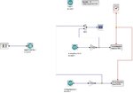
config.jpeg


Code Verilog - [expand]
1
2
3
4
5
6
7
8
9
10
11
12
13
14
15
16
17
18
19
20
21
22
23
24
25
26
27
28
29
30
31
32
33
34
35
36
37
38
39
40
41
42
43
44
45
46
47
48
49
50
51
52
53
54
55
function [Sysc,Hz]=identsys2(u,y,T)
 
    z=%z;
    s=%s


    phi=[];
for i = 1:(length(u)-2)   
    phi = [phi ;y(i+1) y(i)  u(i+1) u(i)];
end
 
Y=(y(3:$));
theta= inv(phi'*phi)*phi'*Y
       disp(theta)
    Hz= (theta(3)*z+theta(4))/(z^2 - theta(1)*z - theta(2))
    
    disp(Hz)
     
    numdeg = degree(Hz.num);
    dendeg = degree(Hz.den);
    if numdeg>dendeg
        error('The discrete-time system is improper');
    end
    f = -(s*T+2);
    g = (s*T-2);
    // extract the coefficients from num and den
    bn = coeff(Hz.num);
    an = coeff(Hz.den);
    npad = dendeg - numdeg;  // number of zero to be padded, if any
    if npad > 0
        for i=0:npad
           bn = [bn 0]; // pad numerator coeff vector with zero 
        end 
    end    
    // The for loop that does the conversion
    nums = 0;
    dens = 0;
    for i=0:dendeg,
       nums = nums + bn(i+1)*(f^i)*(g^(dendeg-i));
       dens = dens + an(i+1)*(f^i)*(g^(dendeg-i));
    end
    Sysc = syslin('c',nums,dens);
    
     coefficients = coeff(Sysc.den)
   //disp(coefficients)  
   common_factor= coefficients(3)
   
   format('v',8)
Sysc.num =  Sysc.num/common_factor
Sysc.den= Sysc.den/common_factor
 
  Sysc.num= clean(Sysc.num,0.1)
   Sysc.den= clean(Sysc.den,0.1)
endfunction

 
Last edited by a moderator:

Could you explain how the estimation is given (which signals you inject, which signals you measure) and the equations you apply ?
 

Could you explain how the estimation is given (which signals you inject, which signals you measure) and the equations you apply ?

I inject from arduino square pulses that rise from 0 to 5 volts and I get them from the digital output pin of arduino. the output that I measure is the output of voltage of the second order under/over damped , and I get it from Analog input of arduino.

the equations that I apply is in the above mentioned code, it is the least square method :


Code Verilog - [expand]
1
2
3
4
5
6
7
8
9
10
11
12
13
14
15
16
17
18
function [Sysc,Hz]=identsys2(u,y,T)
 
    z=%z; // makes z to be dealt as symbol, not as variable
    s=%s; //  makes s to be dealt as symbol, not as variable 


    phi=[];
for i = 1:(length(u)-2)   
    phi = [phi ;y(i+1) y(i)  u(i+1) u(i)];
end
 
Y=y(3:$);   // get Y from third element till end
theta= inv(phi'*phi)*phi'*Y
       disp(theta)
    Hz= (theta(3)*z+theta(4))/(z^2 - theta(1)*z - theta(2))
    
    disp(Hz)

 
Last edited by a moderator:

You did not say if the filters are highpass or lowpass but I assume an RC filter is lowpass.
Maybe the filters attenuate the fundamental frequency of the square waves too much.
Maybe your buffer opamp is not biased correctly or the frequency is too high for it.
Please post the schematic of the filters and opamp (also show its part number) and show the supply voltages (also show the fundamental frequency).
 

OK, what about the gain of your filter ? With a passive network Vo/Vin < 1, but using an opamp you could also have Vo/Vin > 1
 

I am sorry for lack of explanation, I will explain in details what happened, and everyone is invited to tell me his conclusions.
first, I was preparing an experiment for students about basics of system identification, so I began with RC (low pass) passive circuit.

the resistance is 100k and the capacitance is 220 n. I made excitation input as pulses of 5 volts value and frequency of 10 hz. I made the sampling rate of data to be 0.005ms. I got the data between input and output that are in the attached file named "first order".

View attachment first order output.txt
View attachment first order input.txt

I used least square method in the following manner to estimate the parameters:


Code Verilog - [expand]
1
2
3
4
5
6
7
8
9
10
11
12
13
14
15
function [Sysc,Hz]=identsys1(u,y,T)
    z=%z;
    s=%s
 
phi=[];
for i = 1:(length(u)-1)   
    phi = [phi ;y(i)  u(i)];
end
 
Y=y(2:$);
theta= inv(phi'*phi)*phi'*Y
 
disp(theta)
 
     Hz= theta(2)/(z - theta(1))


the rest of code was for making bilinear transformation to get the transfer function again to S domain.


when I used the above mentioned code, I got the estimation of : T.F = 68/(68+s)

and to test the estimated transfer function, I made the following validation in this attached photo:

first order estimated tf vs actual system.jpg


the green curve is the actual response and the red curve is gotten from estimated transfer function. and as it seems it is a perfect estimation.

till now every thing is perfect, and working as it supposed to do.

I made another passive system, RLC, and the results was very good also, only I changed regressor equation (estimation equation) to fit with a second order system instead of first order .

the problems appeared when an opamp is part of the estimated system, even if the opamp is a buffer with nearly no effect at all on circuit performance.


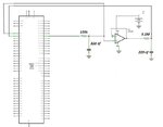
for example, I made double RC circuit in the manner described as follows:

second order schematic.jpg

they are two RC low pass filter circuits, connected with buffering opamp.

the results that I got from estimation are weird and has no relation with the real system.

I recorded the values of input and output in the following attached files (the frequency of input was 10 hz square pulses and the and sampling period was 0.005)

View attachment second order overdamped output.txt
View attachment second order overdamped input.txt

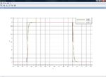
actually, I began to suspect that opamp makes distortion in the signal so the estimated transfer function becomes wrong, so I plotted the signal before opamp and the signal after opamp to see if the opamp makes any effect. please look here:

before opamp vs after opamp.jpg

as we see, no difference that can make wrong estimation.

That is why I got conclusion that existence of opamp makes the estimation process to be wrong, due to unknown reasons.

any suggestions to resolve this weird problem??
 
Last edited by a moderator:

Why is the cutoff frequency of the second RC at 0.143Hz and the cutoff frequency of the first RC far away at 7.3Hz which is 51 times higher than the first? Then it is not a second-order filter and it is not overdamped.

If both RC's are the same then the filter is a second-order with a lot of damping.

Actually, as far as it this system has 2 real poles, then it is a second order system. but I understand your point about that one of them is much bigger than the other so it becomes the "dominant pole", and the system performance tends to be so close to the a first order system that has the dominant pole. but in the end of the day, it is a second order overdamped system with slight s shaped response in the beginning of its response.
in all cases, I tried also to use the poles to be repeated (i.e both R where 100k and both C where 220n) and also I got nearly same problems. I can repeat the experiment and upload its input/output results if needed.
 

Did you try an active Butterworth second-order filter (Sallen and Key type)?

sorry for my late reply. today I could do the same procedure with sallen key filter, but same thing, the identification fails, and it gives me a transfer function of another system that is much slower.

really very strange problem.

let us do a check.

I have put the input output data here in previous post, and I hope that anyone can do parameter estimation procedure using another software (like matlab for example), and tell me the resulting transfer function. I want to know if the problem is in the data aquired or in the software that I am using (scilab), even if this is not logical, because scilab can identify the other first and second order systems that do not contain opamp
 

Status
Not open for further replies.

Part and Inventory Search

Welcome to EDABoard.com

Sponsor

Back
Top