Continue to Site

Welcome to EDAboard.com

Welcome to our site! EDAboard.com is an international Electronics Discussion Forum focused on EDA software, circuits, schematics, books, theory, papers, asic, pld, 8051, DSP, Network, RF, Analog Design, PCB, Service Manuals... and a whole lot more! To participate you need to register. Registration is free. Click here to register now.

Discrete-time step response versus sampling rate question - matlab

Status
Not open for further replies.

SouthPark

Newbie level 6
Joined
Jul 8, 2008
Messages
11
Helped
2
Reputation
4
Reaction score
2
Trophy points
1,283
Activity points
1,427
Hi all! I have a really simple question about understanding matlab plots of a simple step response in discrete-time.

I have a very short matlab (.m file) script that I have attached, where I defined a simple transfer function in the z-domain. A function of 'z'.

And then I just use matlab to plot two STEP responses based on the same transfer function. One response is for sampling period of 1 second, while the other response is for sampling period of 0.1 second.

I was assuming that the two responses would just be super-imposed over each other in the time domain, as I figured that a faster sampling time would simply provide a 'smoother' curve - especially since a smaller sampling period should mean faster sampling rate - and thus a smoother curve.

However, my matlab plots suggest that a faster sampling rate leads to a FASTER response time. I was thinking that a faster sampling rate shouldn't really lead to a faster response time, right? In my matlab plots, it just appears that increasing the sampling rate by a factor of 10 is causing the step response to get quicker (relative to the other plot) by a factor of 10. This doesn't make sense to me, so I thought I'd just ask about this.

Any help is greatly appreciated. Thanks in advance!!
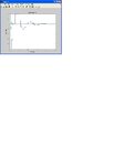
 

Attachments

  • step response plots.JPG
    step response plots.JPG
    52.6 KB · Views: 182
  • step_response_discrete_time.zip
    631 bytes · Views: 96

The result is as expectable. What you want to see, two similar waveforms with different time discretization, would happen if you generate z-domain transfer functions for the same s-domain characteristic with different sampling rates. This results in different sets of z-domain coefficients.
 
Hi FvM! Thanks very very much for helping me. Greatly appreciated. That helped a lot. Before, I kept incorrectly thinking that sampling at a faster rate would yield identical response time, except that one curve would just be blockier and chunkier than the other. That is, I was thinking that faster sampling would just yield a smoother version of the same curve. Your help really steers me in the right direction. Thanks again!
 

The result is as expectable. What you want to see, two similar waveforms with different time discretization, would happen if you generate z-domain transfer functions for the same s-domain characteristic with different sampling rates. This results in different sets of z-domain coefficients.

Hi again FvM!

I was thinking more about what you helped me with, but came across one issue for the case of applying a SINEWAVE input (instead of step input) to the same transfer function.

In my original post - involving STEP responses - I noticed that reducing the sampling period (T) by a factor of 10 led to a step response that occurred more quickly by a factor of 10. That is, the step response with sampling period 0.1 seconds is 10 times slower than the step response with sampling period 0.01 seconds.

However, for the case of a SINEWAVE input, I notice that reducing the sampling period by a factor of 10 did not lead to any 'time compression'. That is, for a sinewave input, the plots with sampling period of 0.1 second and sampling period of 0.01 seconds are basically the same in terms of time-scale.

I'm just having a little trouble in understanding why reducing the sampling period for STEP inputs leads to a time-scale compression, while doing the same thing for SINEwave inputs does not result in any time compression.

Eg...in my attached plots, the sinewave plots match up in time, while the step input plots have same shape but different time-scales.

Thanks FvM.
 

Attachments

  • simulink mdl files with screenshots.zip
    206.3 KB · Views: 80
Last edited:

Update: I understand the situation now. The transfer function (function of Z) has some coefficient values in the polynomials that actually depend on the sampling period T.

This means that if we are given a transfer function (- a function of Z) that ONLY contains z's AND numbers, then it just means that the sampling time T has already been decided upon (chosen). It means that it is tied to some particular value of sampling time already.

Eg... if we start off with G(s) = 1/(s+1), then G(z) = z/[z-e^(-T)], which means that you need to choose a value for 'T' to begin with. So for T = 0.1 second, then G(z)=z/(z-0.9). So in matlab or simulink, if we want the discrete-time STEP response to have the CORRECT time-scale when we use G(z)=z/(z-0.9), then we need to set the sampling time to be 0.1 second.
 
  • Like
Reactions: FvM

    FvM

    Points: 2
    Helpful Answer Positive Rating
Status
Not open for further replies.

Part and Inventory Search

Welcome to EDABoard.com

Sponsor

Back
Top