Continue to Site

Welcome to EDAboard.com

Welcome to our site! EDAboard.com is an international Electronics Discussion Forum focused on EDA software, circuits, schematics, books, theory, papers, asic, pld, 8051, DSP, Network, RF, Analog Design, PCB, Service Manuals... and a whole lot more! To participate you need to register. Registration is free. Click here to register now.

Estimating Frequency Over A Short Capture


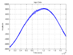
I was recently asked how to estimate the frequency of a noisy sine wave over a short capture. In this context, 'short' means the total capture duration relative to the period of the sine wave. So we may have, at most, a few periods of the sine wave (or, at worst, less than one period). Here is an example (download raw data: View attachment sine_data_40k.zip
):

attachment.php

Clealy, there is less than one period available. To illustrate the difficulty with this problem, I will first describe a popular approach for estimating frequency over 'long' captures.

FFT-based Frequency Estimation ('Long' Captures)

Whenever we are interested in the frequency content of a signal, the Fast Fourier Transform (FFT) is often an excellent tool to use. In practice, when working with real-world (finite and imperfect) data, rather than using the raw output of the FFT, it is often preferable to enhance the FFT's estimate of Power Spectral Density (PSD) using Welch's method, since this can significantly reduce noise (at the expense of reduced resolution).

Here is some Matlab code showing how to use Welch's method to estimate frequency over a 'long' capture (download: View attachment pwelch_test.zip
):


Code Matlab M - [expand]
1
2
3
4
5
6
7
8
9
10
11
12
13
14
15
16
17
18
19
20
21
22
23
24
25
26
27
28
29
30
31
32
33
34
35
close all; clear all; clc;
 
% Assume we capture Nsamps samples at 1kHz sample rate
Nsamps = 32768;
fsamp = 1000;
Tsamp = 1/fsamp;
t = (0:Nsamps-1)*Tsamp;
 
% Assume the noisy signal is exactly 123Hz
fsig = 123;
signal = sin(2*pi*fsig*t);
noise = 1*randn(1,Nsamps);
x = signal + noise;
 
% Plot time-domain signal
subplot(2,1,1);
plot(t, x);
ylabel('Amplitude'); xlabel('Time (secs)');
axis tight;
title('Noisy Input Signal');
 
% Choose FFT size and calculate spectrum
Nfft = 8192;
[Pxx,f] = pwelch(x,gausswin(Nfft),Nfft/2,Nfft,fsamp);
 
% Plot frequency spectrum
subplot(2,1,2);
plot(f,Pxx);
ylabel('PSD'); xlabel('Frequency (Hz)');
grid on;
 
% Get frequency estimate (spectral peak)
[~,loc] = max(Pxx);
FREQ_ESTIMATE = f(loc);
title(['Frequency estimate = ',num2str(FREQ_ESTIMATE),' Hz']);


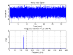
The code outputs this figure:

attachment.php

Although the input looks like a noisy mess, we can see an extremely narrow spike in the spectrum at 123.0469 Hz (i.e. a tiny error of 0.0469 Hz).

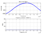
However, if we try the same approach with the 'short' data capture (using this code: View attachment short_pwelch.zip
), we get:

attachment.php

Now the frequency spike is invisible because it is squeezed right down in the first bin after DC. The reason is that, even though I have eliminated any averaging in the Welch method, the frequency bin spacing (i.e. resolution) is still only:

\[\Delta_f = \frac{f_{samp}}{N_{samps}}=50kHz\]​

Therefore, even though the input signal is somewhere in the region of 35kHz, it is impossible for the FFT to provide an answer anywhere between 0 and 50kHz.

It is worth reiterating that the 'short' capture is short in terms of its total duration compared to the period of the sine wave. In fact, there are significantly more samples in the 'short' capture than the 'long' capture, but this doesn't ultimately help.

Frequency Estimation Via Curve Fitting

A far more effective method with 'short' captures is curve fitting. In a previous blog, I wrote about polynomial curve fitting. Well, in this case, we want to do sinusoidal curve fitting. This is easy to do in Matlab, using the 'sin1' option with the fit() function (code: View attachment short_sine_fit.zip
):


Code Matlab M - [expand]
1
2
3
4
5
6
7
8
9
10
11
12
13
14
15
16
17
18
19
20
21
22
close all; clear all; clc;
 
% Load data
load sine_data_40k.dat
x = sine_data_40k;
 
% Data info
Tsamp = 5e-10;
fsamp = 1/Tsamp;
Nsamps = length(x);
t = (0:Nsamps-1).'*Tsamp;
 
% Get sine fit
F = fit(t, x, 'sin1');
 
% Plot data and sine fit
figure();
plot(F,t,x);
grid on;
xlabel('Time (secs)');
ylabel('Amplitude');
title(['Estimated frequency = ', num2str(F.b1/(2*pi)), ' Hz']);


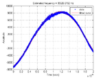
The code outputs this graph:

attachment.php

The frequency estimate of 35526.7 Hz is very much more accurate than the FFT-based method.

Comments

I never thought it was possible to take the spectrum of a signal with only a fraction of its full period.
Thanks for share this work.
 
I like to remind people about significant figures when they talk about accuracy.
35526.7 has only 3 SIG FIGs looking at possible noise error in the graph.

With a signal to noise ratio of < 100:1 and DC offset uncertainty of ~100:1, i.e. 2~3 significant figures.

Using the fundamental slope of the sine wave at zero crossing to the peak or next zero crossing I get 34.0 kHz +/-0.2Hz

Using Irfanview on webimage the time scale 20us was 435 pixels.

So what error do you expect on 35526.7? when I get an optimisitic 34 kHz

7846760700_1417779040.png
 
SunnySkyguy;bt2511 said:
I like to remind people about significant figures when they talk about accuracy.
Why?

SunnySkyguy;bt2511 said:
So what error do you expect on 35526.7? when I get an optimisitic 34 kHz
I don't know what you mean by "optimistic", but I would suggest that your hacky method using lines drawn in an image editor is likely to give very poor estimates, compared to a line-fit derived using proper mathematical rigour. (Not to mention how you would expect to apply your method in a repeatable manner over large data sets). The exact frequency from which this capture was generated was about 35.33kHz. Therefore, the line-fit performs well compared to the FFT-based method in this scenario.

If you are interested in evaluating accuracy in more detail, I would suggest that one easy way of doing this would be to run a large number of trials over synthetic data with known ground truths. As long as your synthetic data has similar statistics to the types of signals you're interested in, then this would answer your question.
 

Part and Inventory Search

Blog entry information

Author
weetabixharry
Read time
3 min read
Views
21,106
Comments
3
Last update

Downloads

  • pwelch_test.zip
    630 bytes · Views: 668
  • short_pwelch.zip
    590 bytes · Views: 685
  • short_sine_fit.zip
    443 bytes · Views: 612
  • sine_data_40k.zip
    15.8 KB · Views: 1,175

More entries in Uncategorized

More entries from weetabixharry

Share this entry

Back
Top